Cavity-Assisted Ion-Photon Emission Simulator

CAIPE-sim is an exploratory tool for studying driven Yb-171 ion–cavity dynamics and supporting hardware-calibration work. Starting from a collaborative three-level cavity-assisted ion–photon entanglement project, I developed the pulse-enabled Yb-171 application around a full 16-state hyperfine basis.

The model combines polarization-resolved laser couplings, independently timed Gaussian drive and repump pulses, and two truncated cavity modes. QuTiP evolves the dissipative system, while an interactive Matplotlib application makes it possible to vary controls and inspect the resulting populations and cavity response.

A three-level Lambda model is a useful starting point for ion–photon dynamics, but a Yb-171 implementation must resolve the hyperfine and magnetic sublevels that determine which transitions each polarization can address. Pulse timing, detuning, magnetic field and loss channels all affect the evolution.

The engineering task was to turn that structure into an inspectable numerical model: map the atomic basis consistently, construct the allowed couplings, evolve time-dependent pulses with dissipation, and expose observables that help explain how a parameter change affects the system.

The atomic basis contains four S states, four P states and eight D states, indexed by manifold, total angular momentum F and magnetic quantum number mF. Electric-dipole coefficients use Wigner 3j and 6j factors to construct separate left, pi and right polarization channels for the S–P drive and D–P repump transitions.

I combine the atomic operators with two finite cavity spaces through tensor products. The Hamiltonian includes laser interactions, cavity coupling, detunings and S/D Zeeman terms. Drive and repump envelopes have independent amplitudes, centers and widths. Collapse operators represent atomic decay, cavity leakage and manifold dephasing, and QuTiP’s master-equation solver computes the dynamics on CPU.

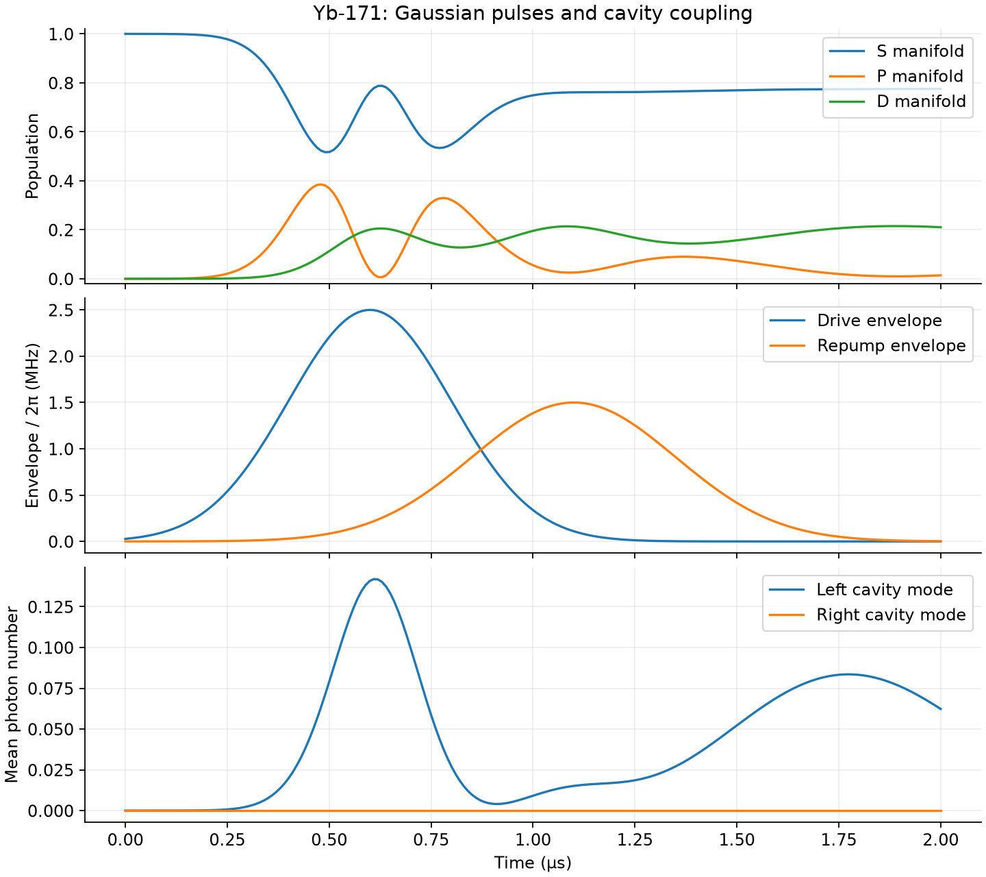
The application exposes pulse, field, polarization, decay and cavity controls through Matplotlib. A separate headless demonstration uses the same backend, starts in S, F=0, mF=0 with empty cavity modes, and exports both a figure and compressed NumPy arrays. Its full manifold projectors account for all 16 atomic states; the interactive application’s three population traces instead represent selected state groups.

My focus was developing the Yb-171 model from the project’s collaborative three-level starting point: expanding the hyperfine basis, constructing polarization-resolved couplings, introducing Gaussian drive and repump pulses, and connecting the dynamics to interactive controls and plots.

The resulting repository brings together the atomic inputs, Hamiltonian and collapse-operator construction, population and cavity observables, and a reproducible CPU demonstration. It also includes numerical checks and documentation of the model conventions and remaining physics questions, so the assumptions can be inspected alongside the output.

The demonstration evolves the 16-state atom with two two-dimensional cavity spaces over 0–2 microseconds, sampling 201 time points. It shows excitation and population transfer during the Gaussian pulses, together with a nonzero response in the selected cavity mode. The exported arrays allow the curves to be analyzed independently of the UI.

The active validation suite checks that the S/P/D projectors partition the basis, that transition coefficients obey selection rules, and that laser and cavity Hamiltonians are Hermitian. It also checks finite, nonnegative observables, conservation of total atomic population and the stationary zero-drive ground-state limit.

An isolated resonant two-level limit compares the numerical response to a Gaussian pulse with the analytic pulse-area Rabi solution, using an absolute tolerance of 2 × 10⁻⁵. The driven demonstration’s population-conservation check uses a tolerance of 10⁻⁶. These are numerical acceptance criteria in the tests, not experimental error estimates.

The outcome is an interactive exploration tool and a reproducible numerical example. The repository does not establish experimental calibration accuracy, photon-generation efficiency or single-photon fidelity. Those require further observable definitions, convergence studies and comparison with the intended experiment.

A consistent basis and explicit conventions are central to this model. The UI uses MHz and microseconds while the solver uses angular frequencies and seconds. Pulse amplitudes pass through scaling and transition-matrix factors, so a slider value must be mapped to a transition-specific Rabi frequency before comparison with experiment. The decay convention follows collapse amplitudes proportional to √(2γ) and √(2κ).

Two cavity spaces are present, but the current polarization branches select one cavity coupling at a time; the pi branch includes neither. Simultaneous evolution of both polarization couplings and the mapping of hyperfine offsets and P-state Zeeman terms remain documented questions for the intended protocol.

Cavity occupation, emitted photon count and the probability of exactly one photon are different observables. A useful output-efficiency study must separate transmission from other losses and integrate the output flux. The UI’s optional static fluorescence correlations also need a time-dependent cavity-output treatment before they can characterize pulsed single-photon emission.

The practical lesson is to validate simple limits before interpreting a complex simulation. Larger cavity truncations and tighter integration settings still need convergence studies, and the older batch implementation needs reconciliation with the active pulse backend before its sweeps can be compared directly.