Distributed Quantum Computing Tutorials

I authored a two-part tutorial series that connects the motivation for distributed quantum computing to the mechanics of distributing a circuit. The first notebook compares monolithic and modular architectures through GHZ circuits, compilation metrics and a simple execution-time model. The second walks through DISQCO using diagrams, a small circuit, a QASM benchmark and a state-movement example.

The materials are designed for hands-on workshop use. Marimo notebooks combine explanations with executable Python, and Jupyter versions provide an alternative format. Readers can inspect intermediate representations, change inputs and reuse the analysis tools for their own circuit families.

Distributed quantum computing introduces a tradeoff between local routing overhead and communication between processors. Explaining that tradeoff requires more than comparing qubit counts: readers need to see what compilation adds, which operations require remote entanglement, and how hardware assumptions affect an execution-time estimate.

Circuit partitioning adds another conceptual gap. A compiler may optimize a temporal hypergraph, but a learner starts with a circuit diagram. The tutorials make those intermediate steps visible so that a partition, its communication cost and the resulting distributed circuit can be understood together.

Notebook 1 starts with a scalable GHZ family. It introduces monolithic compilation using Qiskit’s FakeSherbrooke backend and distributed compilation through the Bosonic SDK, then checks sampled outcomes with Qiskit Aer and the Bosonic simulation path. A shared GateStatistics metric engine compares circuit depth, two-qubit depth, two-qubit counts and total operations.

The notebook builds a timing model from compiled gate counts, gate durations, measurement time and per-shot overhead. It adds an independent-gate success model to estimate success-adjusted time to solution, then fits gate-count trends for larger-size projections. A final exercise lets readers substitute their own measured Qiskit circuit family and reuse the compilation, plotting and modeling functions.

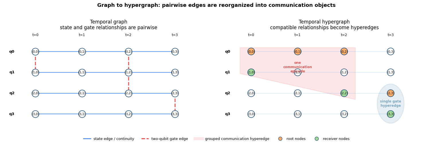
Notebook 2 builds up from graphs and weighted paths to hypergraphs, partition costs and capacity constraints. A four-qubit example shows how a circuit becomes temporal nodes and edges, and how compatible interactions can share a communication episode. The walkthrough then uses DISQCO to partition the 25-qubit knn_n25 benchmark across two QPUs with capacity for 13 logical states each.

A separate synthetic handoff circuit demonstrates time-dependent placement: a hub qubit interacts with one cluster and then another. Readers inspect the assignment matrix, identify state moves and follow extraction into distributed instructions. This complements the benchmark’s static optimized assignment with an example where moving states changes the communication cost.

My contribution is the tutorial narrative and worked examples that connect architecture comparisons to practical circuit distribution. I developed the progression from simple GHZ circuits and explicit modeling assumptions to a guided explanation of DISQCO’s representations, partitioning and circuit extraction.

The material combines explanatory text, circuit diagrams, graph visualizations, tabular metrics and reusable Python helpers. DISQCO and the Bosonic SDK provide the underlying compiler functionality; the tutorial makes their behavior inspectable through concrete examples and exercises.

The saved Jupyter output for knn_n25 compares a naive static placement, DISQCO’s initial placement and the optimized partition. Grouped remote-communication episodes decrease from 37 to 1, while raw remote two-qubit gates decrease from 72 to 24. These are different metrics: a group can cover several compatible gates. The figures describe this recorded example, rather than a general compiler speedup.

In the saved synthetic handoff example, the optimized assignment exchanges two logical states between QPUs. Its reported hypergraph cost falls from 12 to 2, with two state moves and no cut gate/group episodes. The extracted circuit includes entanglement-generation, measurement, reset and correction operations, showing how an abstract placement becomes a distributed program.

The first notebook checks that GHZ samples lie in the expected all-zero and all-one outcomes and are approximately balanced. This is a useful measurement-distribution check, but it is not a full state-fidelity or coherence test. Its timing and utility-scale plots are model-based estimates and extrapolations, not measurements on a large distributed quantum computer.

The delivered outcome is a pair of workshop tutorials with executable examples, saved Jupyter outputs and an extension exercise. The repository does not report measured learning outcomes; its concrete evidence is the material itself and the intermediate compiler outputs that readers can inspect.

GHZ circuits keep the opening comparison understandable: adding a qubit adds a predictable logical interaction. That simplicity also limits what can be inferred about other algorithms. The custom-circuit exercise turns the initial example into a starting point for investigation rather than a universal scaling claim.

I separate gate counts from hardware timing assumptions. The timing model assumes sequential gates and independent gate errors, while the distribution walkthrough assumes unrestricted inter-QPU links and local connectivity and treats entanglement generation as a black box. Those choices support intuition, but scheduling, link contention and noise correlations need more detailed treatment for hardware predictions.

The visual progression is equally important: circuit, temporal graph, grouped hypergraph, assignment matrix and extracted instructions each answer a different question. Keeping a small example through the early transformations makes communication reuse easier to follow before introducing a larger benchmark.

Reproducibility extends beyond exporting a notebook. The repository documents Marimo dependency sandboxes and Jupyter conversion, but parts of the second tutorial still rely on local helpers and an external compiler checkout for its final comparison table. A fresh environment needs those paths and dependencies checked before a workshop run.